sItô compiles system of stochastic differential equations into a Monte Carlo simulation of it that runs fast and can be differentiated with respect to the parameters involved. It does this by joining four ideas: the symbolic calculus of SDEs, their numerical schemes, code generation from symbolic expressions, and automatic differentiation. The interactive demo is at ito.muoperator.com
The starting point is a chapter by Cyganowski, Grüne and Kloeden on a Maple package for SDEs [1] wherein the authors turns the calculus of Itô and Stratonovich equations into symbolic operations. This work can be seen as adding experimental layers on that basis to define high speed simulations, automated differentiation and a useful domain specific language to express the results we are interested in.
1. Itô processes
The state $X_t \in \mathbb{R}^d$ is driven by an $m$-dimensional Wiener process
$$W_t = (W^1_t, \dots, W^m_t)$$with independent components. The dynamics is completely described by the drift $a\colon [0,T]\times\mathbb{R}^d \to \mathbb{R}^d$ and the diffusion $b\colon [0,T]\times\mathbb{R}^d \to \mathbb{R}^{d\times m}$ and can be written in matrix form as
$$ dX_t = a(t, X_t)\,dt + b(t, X_t)\,dW_t, $$or component-wise as,
$$ dX^k_t = a^k(t, X_t)\,dt + \sum_{j=1}^{m} b^{k,j}(t, X_t)\,dW^j_t, \quad k = 1,\dots,d $$Formally this is not a differential equation but just shorthand for an integral equation
$$ \begin{aligned} X^k_t ={}& X^k_{t_0} \\ &+ \int_{t_0}^{t} a^k(s, X_s)\,ds \\ &+ \sum_{j=1}^{m} \int_{t_0}^{t} b^{k,j}(s, X_s)\,dW^j_s , \end{aligned} $$in which the stochastic integrals are Itô integrals. The same process can be written with Stratonovich integrals, $\circ\,dW^j_s$, and then has a different drift. The drift of the Itô form is
$$ a^k_{\text{Itô}} = a^k_{\text{Strat}} + \tfrac12 \sum_{j=1}^{m} \sum_{l=1}^{d} b^{l,j}\,\partial_l b^{k,j} $$for $k = 1,\dots,d$. Which form a model is written in is a modelling choice. The numerical schemes below are derived for the Itô form, so a Stratonovich model is converted first and simulated as its Itô equivalent.
2. Itô’s Lemma
Let $U(t,x)$ be a function of $t$ and $x \in \mathbb{R}^d$ that is once continuously differentiable in $t$ and twice in $x$. Two operators do most of the work. For $j = 1,\dots,m$,
$$ L^j U = \sum_{k=1}^{d} b^{k,j}\,\partial_k U , $$and
$$ \begin{aligned} L^0 U ={}& \partial_t U \\ &+ \sum_{k=1}^{d} a^k\,\partial_k U \\ &+ \tfrac12 \sum_{j=1}^{m} \sum_{k=1}^{d} \sum_{l=1}^{d} b^{k,j}\,b^{l,j}\,\partial_k \partial_l U . \end{aligned} $$The inner sum in the drift correction of the previous section is $L^j b^{k,j}$. In these terms Itô’s Lemma reads:
Itô’s Lemma. If $X$ solves the equation of section 1, then for $s \le t$
$$ \begin{aligned} U(t, X_t) ={}& U(s, X_s) \\ &+ \int_s^t L^0 U(r, X_r)\,dr \\ &+ \sum_{j=1}^{m} \int_s^t L^j U(r, X_r)\,dW^j_r . \end{aligned} $$A transformed process $Y_t = U(t, X_t)$ is therefore an Itô process with drift $L^0 U$ and diffusion columns $L^j U$. Itô’s lemma is the chain rule of stochastic calculus.
Example For geometric Brownian motion, $d = m = 1$, and $U = ln$
$$dX = \mu X\,dt + \sigma X\,dW,$$the operators give
$$ \begin{aligned} L^0 U &= \mu - \tfrac{\sigma^2}{2} , \\ L^1 U &= \sigma , \end{aligned} $$and therefore by Itô’s Lemma
$$ d\ln X_t = \left(\mu - \tfrac{\sigma^2}{2}\right) dt + \sigma\,dW_t . $$The crucial point here is that every step is a symbolic operation on expressions: differentiate, multiply, sum. sItô does them symbolically and keeps the transformed equation in symbolic form, with the parameters still symbols. This matters later for two reasons. The schemes need the derivatives $L^{j_1} b^{k,j_2}$ of the coefficients, and they get them exactly. And the parameters stay visible to the rest of the pipeline, which is what makes derivatives with respect to them possible.
3. Discretization: recursive equations
A scheme is a rule that advances the process from $t_n$ to $t_{n+1} = t_n + \Delta$. It can be derived from the integral equation in one substitution. Over one step, for $k = 1,\dots,d$,
$$ \begin{aligned} X^k_{n+1} ={}& X^k_n \\ &+ \int_{t_n}^{t_{n+1}} a^k(s, X_s)\,ds \\ &+ \sum_{j=1}^{m} \int_{t_n}^{t_{n+1}} b^{k,j}(s, X_s)\,dW^j_s . \end{aligned} $$Apply the Itô formula to $a^k(s, X_s)$ between $t_n$ and $s$,
$$ \begin{aligned} a^k(s, X_s) ={}& a^k(t_n, X_n) \\ &+ \int_{t_n}^{s} L^0 a^k(r, X_r)\,dr \\ &+ \sum_{j=1}^{m} \int_{t_n}^{s} L^j a^k(r, X_r)\,dW^j_r , \end{aligned} $$and in the same way to $b^{k,j}(s, X_s)$, and insert both. With $a^k$ and $b^{k,j}$ now evaluated at $(t_n, X_n)$ and
$$ \Delta W^j = W^j_{t_{n+1}} - W^j_{t_n} , $$the result is
$$ X^k_{n+1} = X^k_n + a^k\,\Delta + \sum_{j=1}^{m} b^{k,j}\,\Delta W^j + R^k . $$The remainder $R^k$ consists of four double integrals,
$$ \begin{aligned} R^k ={}& \iint L^0 a^k\,dr\,ds \\ &+ \sum_{j=1}^{m} \iint L^j a^k\,dW^j_r\,ds \\ &+ \sum_{j=1}^{m} \iint L^0 b^{k,j}\,dr\,dW^j_s \\ &+ \sum_{j_1=1}^{m} \sum_{j_2=1}^{m} \iint L^{j_1} b^{k,j_2}\,dW^{j_1}_r\,dW^{j_2}_s , \end{aligned} $$each over $t_n \le r \le s \le t_{n+1}$, with the integrands evaluated along the path. The first three are of size $\Delta^2$ or $\Delta^{3/2}$. The last is of size $\Delta$. Dropping $R^k$ gives the Euler scheme,
$$ X^k_{n+1} = X^k_n + a^k\,\Delta + \sum_{j=1}^{m} b^{k,j}\,\Delta W^j . $$Keeping the last term, with its integrand frozen at $(t_n, X_n)$, gives the Milstein scheme,
$$ \begin{aligned} X^k_{n+1} ={}& X^k_n \\ &+ a^k\,\Delta \\ &+ \sum_{j=1}^{m} b^{k,j}\,\Delta W^j \\ &+ \sum_{j_1=1}^{m} \sum_{j_2=1}^{m} L^{j_1} b^{k,j_2}\,I_{(j_1, j_2)} , \end{aligned} $$with the iterated integrals
$$ I_{(j_1, j_2)} = \int_{t_n}^{t_{n+1}} \int_{t_n}^{s} dW^{j_1}_r\,dW^{j_2}_s . $$Repeating the substitution gives the Itô-Taylor expansion, and the higher schemes are its truncations [2]. The expansion is generated by the same two operators, which is why a symbolic implementation of $L^0$ and $L^j$ is enough to derive any of them.
Two properties decide what a scheme costs and what it is good for.
Strong and weak order. A scheme has strong order $\gamma$ if
$$ \mathbb{E}\,\bigl|X_T - X^\Delta_T\bigr| \le C\,\Delta^{\gamma} , $$and weak order $\beta$ if, for smooth $f$,
$$ \bigl|\mathbb{E} f(X_T) - \mathbb{E} f(X^\Delta_T)\bigr| \le C\,\Delta^{\beta} . $$Strong order is accuracy of the path. Weak order is accuracy of expectations, which is what prices and moments need.
Iterated integrals. For $j_1 = j_2 = j$ the integral has a closed form,
$$ I_{(j,j)} = \tfrac12 \left( (\Delta W^j)^2 - \Delta \right) . $$For one noise term, Milstein becomes the familiar
$$ X_{n+1} = X_n + a\,\Delta + b\,\Delta W + \tfrac12\,b\,b' \left( (\Delta W)^2 - \Delta \right) . $$For $j_1 \ne j_2$ the integrals are Lévy areas. They have no closed form in terms of the increments. Only their sum has one,
$$ I_{(j_1, j_2)} + I_{(j_2, j_1)} = \Delta W^{j_1}\,\Delta W^{j_2} . $$In the demo, models with one noise term or with diagonal noise run without the Lévy areas. For the other cases there are provisions to supply the integrals, outside the demo.
| Scheme | Order | Needs beyond $\Delta W$ |
|---|---|---|
| Euler | strong 0.5 | nothing |
| Milstein | strong 1.0 | the double integrals $I_{(j_1,j_2)}$ |
| Strong Taylor 1.5 | strong 1.5 | further time integrals and triple integrals |
| Weak Euler | weak 1.0 | nothing |
| Weak Taylor 2.0 | weak 2.0 | its own double integrals |
4. From the recursion to a program
A recursion
$$ x_{n+1} = \Phi_\theta(t_n, x_n, \Delta W_n) , \qquad x_n \in \mathbb{R}^d , \ \Delta W_n \in \mathbb{R}^m , $$with parameters $\theta \in \mathbb{R}^p$ is a function. A Monte Carlo simulation applies the same function to many independent noise sequences, one per path. The paths do not depend on each other, so they form a batch, and the time steps form a loop.
sItô generates the program for the scheme that was chosen, not for the equation alone. The scheme decides which terms exist: Milstein has the $L^{j_1} b^{k,j_2}$ terms, the strong order 1.5 scheme has more. The program is generated after the discretisation, from the symbolic coefficients, and compiled for the machine. The combination of the loop over time and the batch of paths is arranged so that it runs fast and in parallel.
Compiling and simulating are two separate steps. The description of the model, the scheme and the time grid are compiled once into a program. The program is then run with the initial values, the parameter values and a seed as arguments, as often as wanted and without compiling again. A compile takes about half a second; a run takes a few milliseconds (medians of 482 ms and 2 ms on the demo host).
5. What is asked of the paths
A simulation produces paths. What a user wants from them is a handful of numbers or pictures: the distribution of the final value, the mean of a payoff, the fan of paths over time. sItô has a thin language for this. A model is written as formulas, and the questions are lines of that language. Take an Asian call, a payoff that depends on the whole path through the average of the price,
$$ dX = r X\,dt + \sigma X\,dW , $$and
$$ Y = \left( \int_0^T X\,dt - K \right)^{+} . $$The input is
state variable    x
parameters        r, sigma, k
drift             r * x
diffusion         sigma * x
transform         y = max(Integral(x) - k, 0)
statistics        Path(y)
                  Terminal(y)
                  Mean(y)
Integral(x) is a quantity accumulated along each path. Path(y) asks for the evolution of $y$ over time, Terminal(y) for its value at $T$, Mean(y) for its mean. Other lines ask for the maximum over the path or for a first-passage time.
The lines are compiled into the same program as the scheme. Quantities that are accumulated along a path, such as an integral, a maximum or a first passage, are computed while the path is generated. Whatever is not asked for is not kept, so memory follows what is asked for and not the number of paths times the number of steps, and the run is cheaper because nothing is produced that nobody reads.
One argument: a distribution over the paths. Path(y) asks for the distribution of $y$ over the paths at every time. The result is a fan: the density of the paths, with their mean, median and the 5% and 95% quantiles. For the Asian call it shows how the payoff builds up along the path.
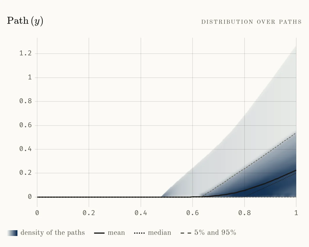
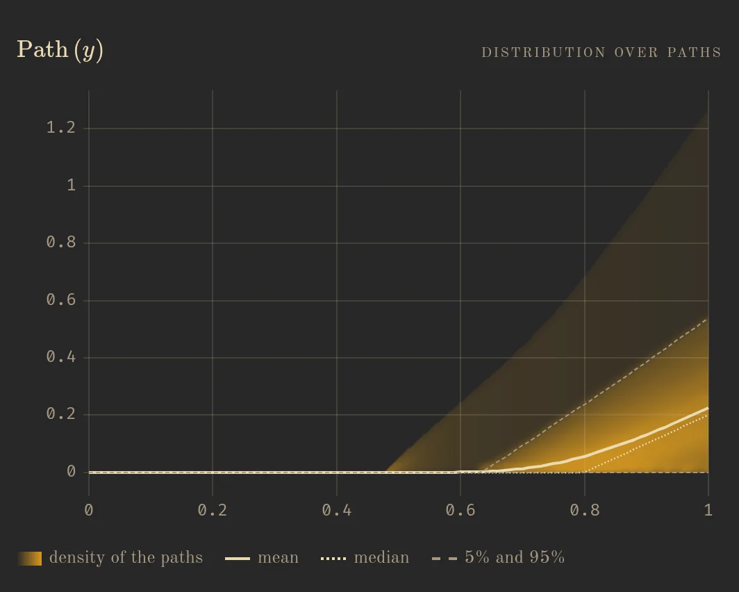
Path(y) for the Asian call: the density of the paths over time, with mean, median and the 5% and 95% quantiles. Parameters $r = 0.03$, $\sigma = 0.3$, $K = 0.8$; 10,000 paths, 100 Euler steps, $T = 1$. The payoff stays at zero until the average of the price can exceed $K$. Experiment with this setting.Terminal(x) asks for the distribution of the value at the final time. For geometric Brownian motion it is the log-normal density.
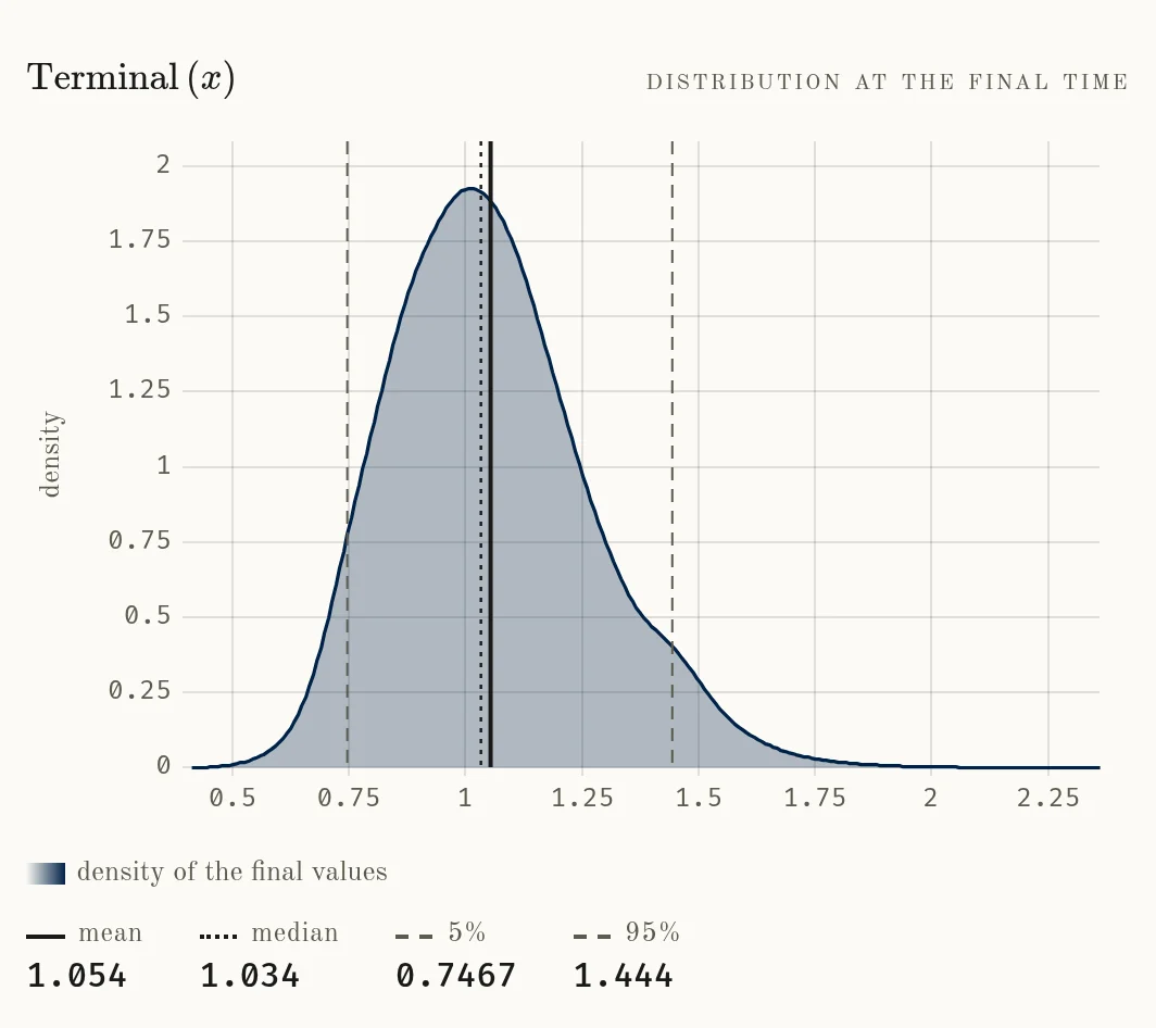
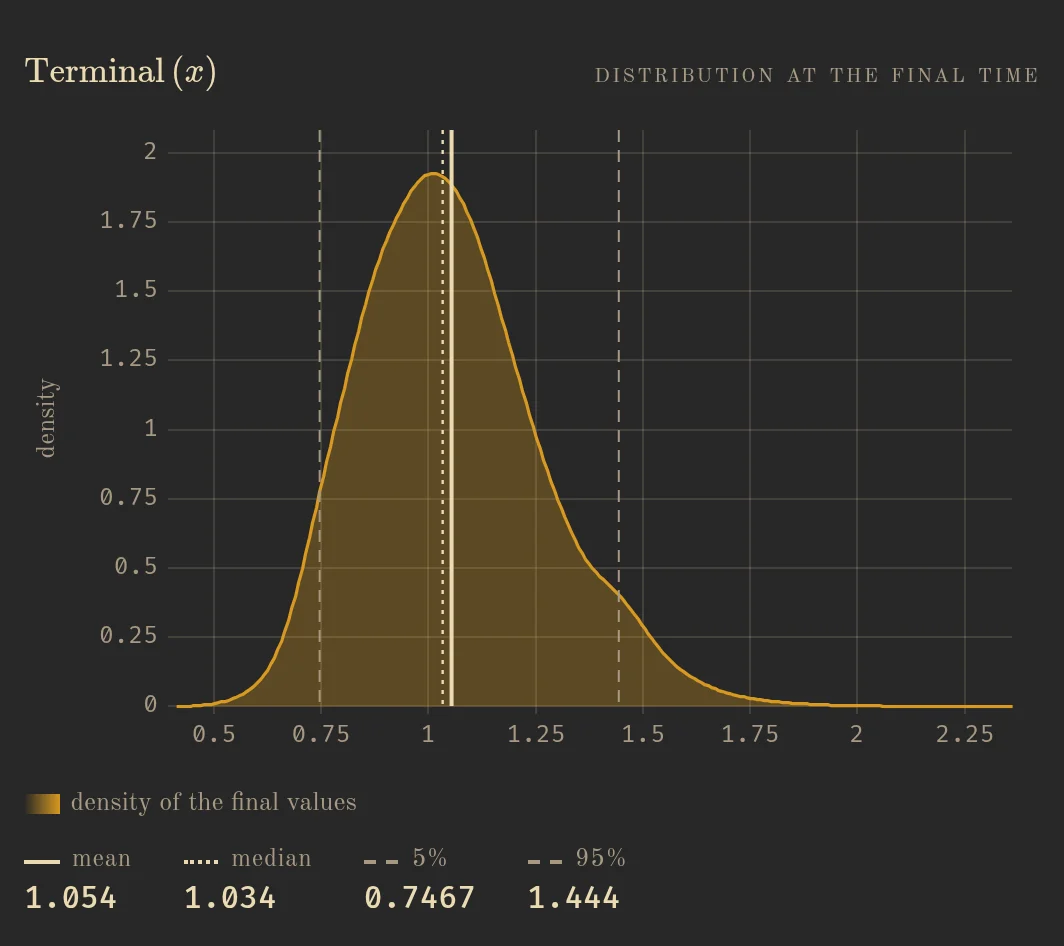
Terminal(x) for geometric Brownian motion: the density of the final values, with mean, median and the 5% and 95% quantiles. Experiment with this example.Several arguments: the paths themselves. With two or three arguments the same word asks a different question. It no longer asks for the distribution of each quantity over time. It asks where the process goes. Path(x, y) draws the individual paths in the $x$–$y$ plane. Path(x, y, z) shows the three projections. A distribution over the paths needs many paths. A trajectory needs only a few, and many time steps. When every statistics line of a model is of this kind, sItô changes the simulation to match: five paths, up to 4,000 time steps and a horizon up to $T = 40$, instead of thousands of paths.
With two arguments, the coupled pair $dX = a(Y - X)\,dt + sX\,dW^1$, $dY = (bX - Y)\,dt + rY\,dW^2$ is the smallest example.
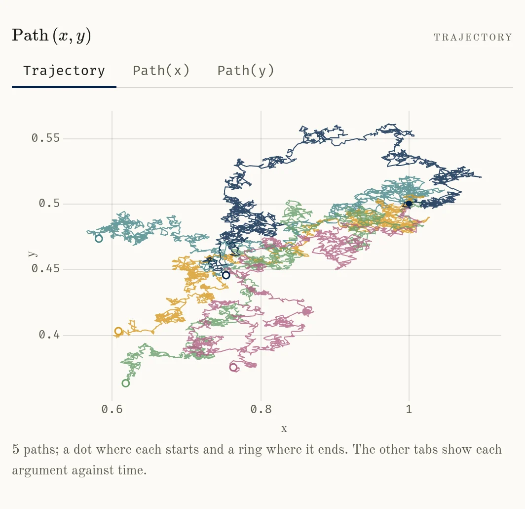
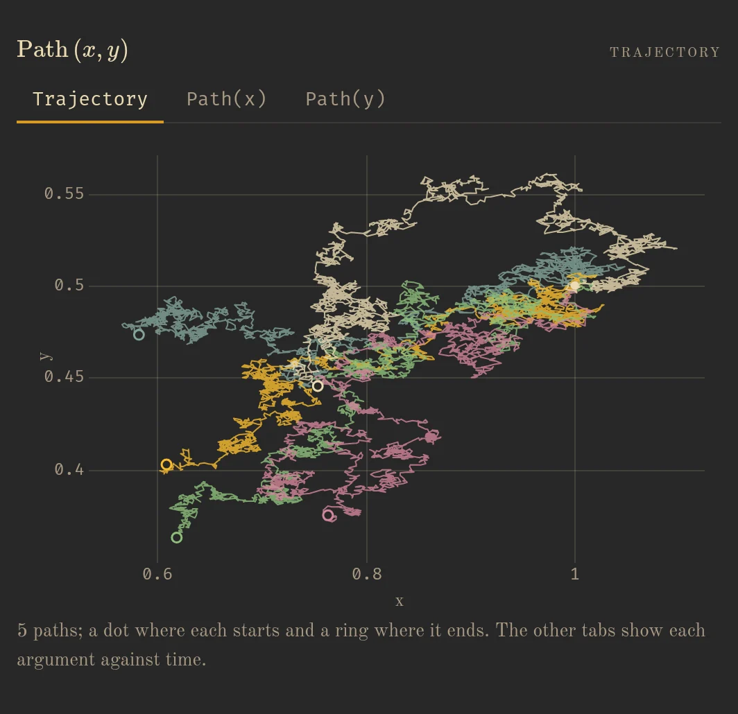
Path(x, y) for the coupled pair: five paths in the $x$–$y$ plane, 2,000 time steps, $T = 1$; a dot marks where each path starts and a ring where it ends. Experiment with this example.With three arguments, the stochastic Lorenz system, $d = m = 3$, shows the familiar two lobes.
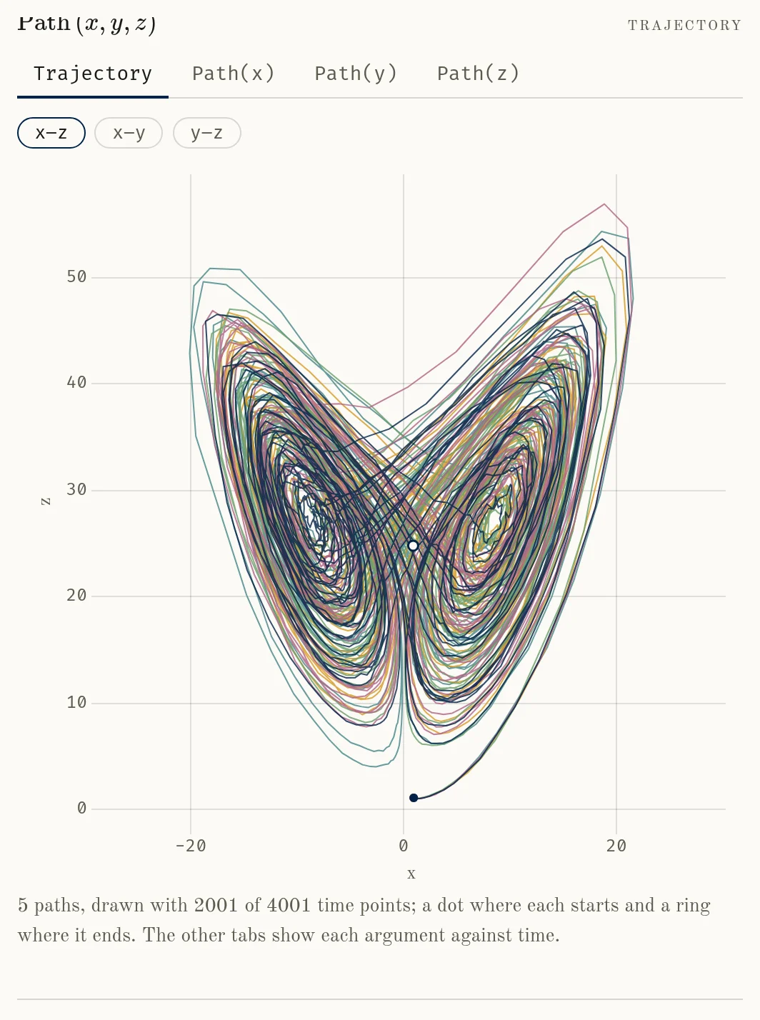
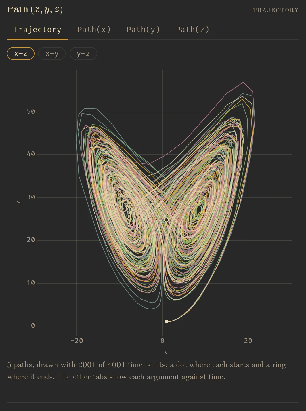
Path(x, y, z) for the stochastic Lorenz system: five paths of 4,000 time steps, $T = 40$, projected on the $x$–$z$ plane. The other tabs show each argument against time. Experiment with this example.6. Derivatives with respect to the parameters
Since the SDE parameters are symbols and the program is a function of them, the generated program can be differentiated by AD. For a fixed noise sequence the simulated value $f(X_T^\theta)$ is a function of $\theta$, and its derivative is computed together with the value.
This is the pathwise estimator, for $i = 1,\dots,p$,
$$ \partial_{\theta_i}\,\mathbb{E}\,f(X_T^\theta) = \mathbb{E}\,\partial_{\theta_i} f(X_T^\theta) , $$applied to the discretised scheme. It holds under regularity conditions, for example for a payoff that is Lipschitz and a scheme that is smooth in $\theta$. The Asian call above satisfies them for the first derivatives. A discontinuous payoff, such as a digital option, does not, and neither do second derivatives of a call. Those need other methods.
Note that we could have alternatively computed the symbolic derivative of the expression and then generate the equivalent program. While correct this has drawbacks when we need to compute derivatives with respect to several parameters.
7. Tests and Demo Limits
The schemes are checked against the theory in two ways. The convergence orders are measured on models with known solutions: Euler converges at strong order 0.5, and the strong order 1.5 scheme measures between 1.4 and 2.1 on the test models. And the models with a closed form, such as geometric Brownian motion, the Ornstein-Uhlenbeck process and others, are compared with it: mean, variance and terminal distribution. A Stratonovich model is checked against its converted Itô form.
The demo enforces several limits to control used resources. The strong schemes with cross terms need the Lévy areas, which the demo does not offer.
The interactive application is at ito.muoperator.com.
References
- S. Cyganowski, P. Kloeden, L. Grüne, MAPLE for Stochastic Differential Equations, in J. Blowey, J. Coleman, A. Craig (eds.), Theory and Numerics of Differential Equations: Durham 2000, Springer, 2001, chapter 1.
- P. E. Kloeden, E. Platen, Numerical Solution of Stochastic Differential Equations, Springer, 1992.